Microsoft Excel pivot table

A pivot table allows you to extract the significance from a large, detailed data set.

Our data set consists of 214 rows and 5 fields. Sl no, Product, Area, Amount, Date.

Insert a Pivot Table

To insert a pivot table, execute the following steps.

1. Click any single cell inside the data set.

2. On the Insert tab, click PivotTable.

The following dialog box appears. Excel automatically selects the data for you. The default location for a new pivot table is New Worksheet.

3. Click OK.

Drag fields

The PivotTable field list appears. To get the total amount exported of each product, drag the following fields to the different areas.

1. Product Field to the Row Labels area.

2. Amount Field to the Values area.

Below you can find the pivot table. Bananas are our main export product. That's how easy pivot tables can be!

Filter

Now we filter the data's based on product wise sold area.

1. Drag the Product from ROWS to Filter, and drag the area to ROWS column.

Result. Area wise main export product to Fridge.

Note: you can use the standard filter (triangle next to Product) to only show the totals of specific products.

Change Summary Calculation

By default, Excel summarizes your data by either summing or counting the items. To change the type of calculation that you want to use, execute the following steps.

1. Click any cell inside the Total column.

2. Right click and click on Value Field Settings...

3. Choose the type of calculation you want to use. For example, click Count.

4. Click OK.

Result. 16 out of the 28 orders to Fridge were 'Frazer town' orders.

Two-dimensional Pivot Table

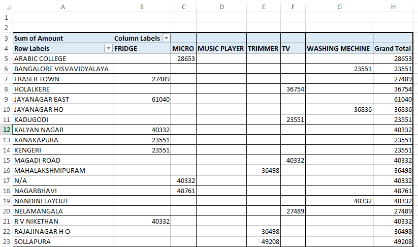
If you drag a field to the Row Labels area and Column Labels area, you can create a two-dimensional pivot table. For example, to get the total amount exported to each country, of each product, drag the following fields to the different areas.

1. Area Field to the Row Labels area.

2. Product Field to the Column Labels area.

3. Amount Field to the Values area.